Comparative Analysis of Classification Algorithms
June 2020
2840 Words, 16 Minutes
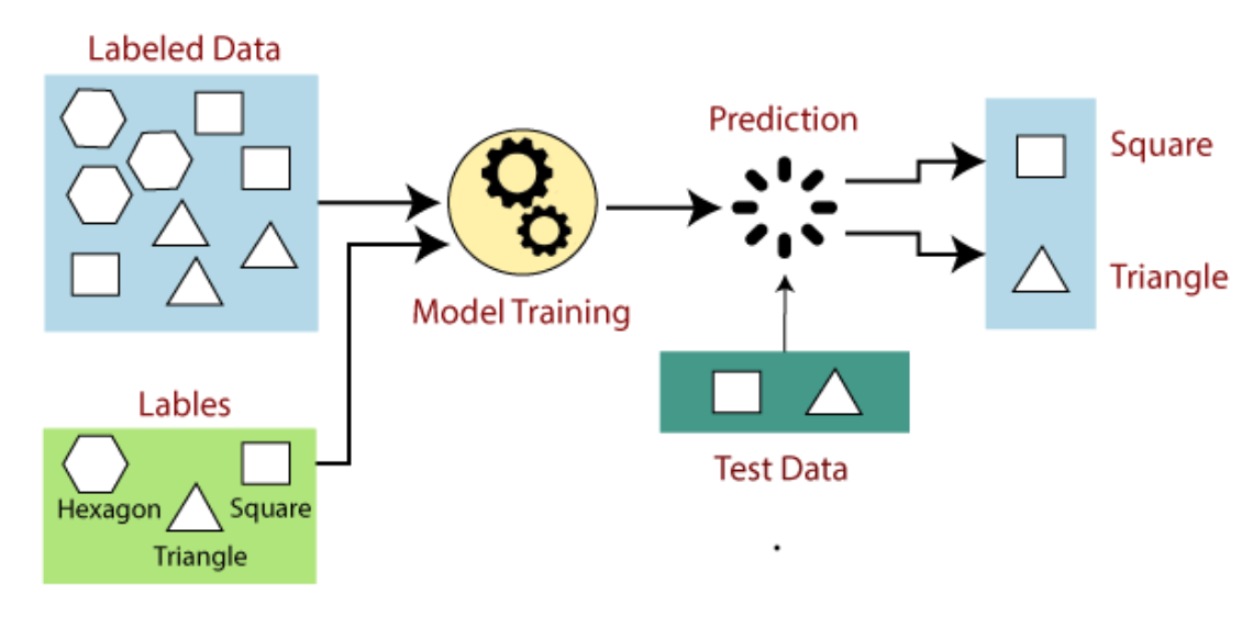
Supervised Machine Learning Algorithms
Supervised learning is the types of machine learning in which machines are trained using well “labelled” training data, and on basis of that data, machines predict the output. The labelled data means some input data is already tagged with the correct output. In supervised learning, the training data provided to the machines work as the supervisor that teaches the machines to predict the output correctly. It applies the same concept as a student learns in the supervision of the teacher. Supervised learning is a process of providing input data as well as correct output data to the machine learning model. The aim of a supervised learning algorithm is to find a mapping function to map the input variable(x) with the output variable(y). In the real-world, supervised learning can be used for Risk Assessment, Image classification, Fraud Detection, spam filtering, etc.
Algorithms I have implemented are:
- K-Nearest Neighbour
- Random Forest
- Decision Tree
- Support Vector Machine
Importing Libraries
We will import the necessary libraries that we will need in our project.
- Label Encoder a popular encoding technique for handling categorical variables
- Stanndard Scaler is used to normalize the values
- Simple Imputer is used to fill in missing values
- Seaborn is used for data visualisation
 import pandas as pd
from sklearn.preprocessing import LabelEncoder
from sklearn.preprocessing import StandardScaler
from sklearn.impute import SimpleImputer
from sklearn.neighbors import KNeighborsClassifier
from sklearn.model_selection import train_test_split
from sklearn.metrics import confusion_matrix
from sklearn.metrics import accuracy_score
import matplotlib.pyplot as plt
from sklearn.ensemble import RandomForestClassifier
import seaborn as sn
from sklearn.tree import DecisionTreeClassifier
from sklearn import svm
import seaborn as sns
Reading the csv
We have taken the dataset of a Liver Patient.Based on chemical compounds(bilrubin,albumin,protiens,alkaline phosphatase) present in human body and tests like SGOT , SGPT the outcome mentioned whether person is patient ie needs to be diagnosed or not.
 df = pd.read_csv("data1/liver_p.csv")
df.head()
Output
Age	Gender	Total_Bilirubin	Direct_Bilirubin	Alkaline_Phosphotase	Alamine_Aminotransferase	Aspartate_Aminotransferase	Total_Protiens	Albumin	Albumin_and_Globulin_Ratio	Dataset
0	65	Female	0.7	0.1	187	16	18	6.8	3.3	0.90	1
1	62	Male	10.9	5.5	699	64	100	7.5	3.2	0.74	1
2	62	Male	7.3	4.1	490	60	68	7.0	3.3	0.89	1
3	58	Male	1.0	0.4	182	14	20	6.8	3.4	1.00	1
4	72	Male	3.9	2.0	195	27	59	7.3	2.4	0.40	1
Checking for missing values
X = df[features]
Y = df.Dataset
df.isnull().sum()
Output
Age                           0
Gender                        0
Total_Bilirubin               0
Direct_Bilirubin              0
Alkaline_Phosphotase          0
Alamine_Aminotransferase      0
Aspartate_Aminotransferase    0
Total_Protiens                0
Albumin                       0
Albumin_and_Globulin_Ratio    4
Dataset                       0
dtype: int64
Since there are missing values we will handle them using the Simple Imputer library and fill in the mean of the column for the missing value
imp = SimpleImputer(strategy ="mean")
X_new =pd.DataFrame(imp.fit_transform(X))
X_new.columns = df[features].columns
X_new.head()
Output
	Age	Gender	Total_Bilirubin	Direct_Bilirubin	Alkaline_Phosphotase	Alamine_Aminotransferase	Aspartate_Aminotransferase	Total_Protiens	Albumin	Albumin_and_Globulin_Ratio
0	65.0	0.7	0.1	187.0	16.0	18.0	6.8	3.3	0.90	0.0
1	62.0	10.9	5.5	699.0	64.0	100.0	7.5	3.2	0.74	1.0
2	62.0	7.3	4.1	490.0	60.0	68.0	7.0	3.3	0.89	1.0
3	58.0	1.0	0.4	182.0	14.0	20.0	6.8	3.4	1.00	1.0
4	72.0	3.9	2.0	195.0	27.0	59.0	7.3	2.4	0.40	1.0
Checking for missing values again
X_new.isnull().sum()
Output
Age                           0
Gender                        0
Total_Bilirubin               0
Direct_Bilirubin              0
Alkaline_Phosphotase          0
Alamine_Aminotransferase      0
Aspartate_Aminotransferase    0
Total_Protiens                0
Albumin                       0
Albumin_and_Globulin_Ratio    0
dtype: int64
Dropping the Gender Column
X.drop("Gender" , axis = 1 , inplace = True )
X.head()
Output
Age	Total_Bilirubin	Direct_Bilirubin	Alkaline_Phosphotase	Alamine_Aminotransferase	Aspartate_Aminotransferase	Total_Protiens	Albumin	Albumin_and_Globulin_Ratio	Sex
0	65	0.7	0.1	187	16	18	6.8	3.3	0.90	0
1	62	10.9	5.5	699	64	100	7.5	3.2	0.74	1
2	62	7.3	4.1	490	60	68	7.0	3.3	0.89	1
3	58	1.0	0.4	182	14	20	6.8	3.4	1.00	1
4	72	3.9	2.0	195	27	59	7.3	2.4	0.40
Data Visualisation
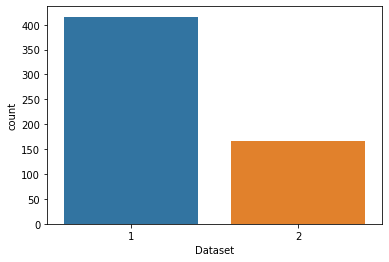
We will visualise the patients having the liver disease and the ones not having the disease.
sns.countplot(data=df, x = 'Dataset', label='Count')

LD, NLD = df['Dataset'].value_counts()
print('Number of patients diagnosed with liver disease: ',LD)
print('Number of patients not diagnosed with liver disease: ',NLD)
Output
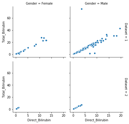
Mapping one feature with respect to another using seaborn library
g = sns.FacetGrid(df, col="Gender", row="Dataset", margin_titles=True)
g.map(plt.scatter,"Direct_Bilirubin", "Total_Bilirubin", edgecolor="w")
plt.subplots_adjust(top=0.9)
Output
Data Normalisation
Normalization is generally required when we are dealing with attributes on a different scale, otherwise, it may lead to a dilution in effectiveness of an important equally important attribute(on lower scale) because of other attribute having values on larger scale. In simple words, when multiple attributes are there but attributes have values on different scales, this may lead to poor data models while performing data mining operations. So they are normalized to bring all the attributes on the same scale.
X_arr = X_new.iloc[: , : ]
Y_arr = df.iloc[: , -1]
sc = StandardScaler()
X_arr = sc.fit_transform(X_arr)
X_arr
Output
array([[ 1.25209764, -0.41887783, -0.49396398, ...,  0.19896867,
        -0.14789798, -1.76228085],
       [ 1.06663704,  1.22517135,  1.43042334, ...,  0.07315659,
        -0.65069686,  0.56744644],
       [ 1.06663704,  0.6449187 ,  0.93150811, ...,  0.19896867,
        -0.17932291,  0.56744644],
       ...,
       [ 0.44843504, -0.4027597 , -0.45832717, ...,  0.07315659,
         0.16635131,  0.56744644],
       [-0.84978917, -0.32216906, -0.35141677, ...,  0.32478075,
         0.16635131,  0.56744644],
       [-0.41704777, -0.37052344, -0.42269037, ...,  1.58290153,
         1.73759779,  0.56744644]])
Splitting the data into train and test set
ain-Valid-Test split is a technique to evaluate the performance of your machine learning model — classification or regression alike. Train Dataset
- Set of data used for learning (by the model), that is, to fit the parameters to the machine learning model Valid Dataset
- Set of data used to provide an unbiased evaluation of a model fitted on the training dataset while tuning model hyperparameters.
- Also play a role in other forms of model preparation, such as feature selection, threshold cut-off selection. Test Dataset
- Set of data used to provide an unbiased evaluation of a final model fitted on the training dataset.
X_train , X_test , Y_train , Y_test = train_test_split(X_arr , Y_arr , test_size = 0.2 , shuffle = True)
len(X_train) , len(X_test) , len(Y_train) , len(Y_test)
Output
(466, 117, 466, 117)
Building K-Nearest Neighbour Model
K-Nearest Neighbours is one of the most basic yet essential classification algorithms in Machine Learning. It belongs to the supervised learning domain and finds intense application in pattern recognition, data mining and intrusion detection. It is widely disposable in real-life scenarios since it is non-parametric, meaning, it does not make any underlying assumptions about the distribution of data.
Algorithm
- Let m be the number of training data samples. Let p be an unknown point.
- Store the training samples in an array of data points arr[]. This means each element of this array represents a tuple (x, y).
- for i=0 to m: Calculate Euclidean distance d(arr[i], p).
- Make set S of K smallest distances obtained. Each of these distances corresponds to an already classified data point.
- Return the majority label among S.
model_knn = KNeighborsClassifier(n_neighbors= 3)
model_knn.fit(X_train , Y_train)
pred = model_knn.predict(X_test)
score = accuracy_score(pred , Y_test)
score
Output
KNeighborsClassifier(algorithm='auto', leaf_size=30, metric='minkowski',
                     metric_params=None, n_jobs=None, n_neighbors=3, p=2,
                     weights='uniform')
Output
0.6324786324786325
cm = confusion_matrix(Y_test , pred)
print(cm)
Output
[[64 18]
 [25 10]]
Building Random Forest Classifier
The Random forest or Random Decision Forest is a supervised Machine learning algorithm used for classification, regression, and other tasks using decision trees. The Random forest classifier creates a set of decision trees from a randomly selected subset of the training set. It is basically a set of decision trees (DT) from a randomly selected subset of the training set and then It collects the votes from different decision trees to decide the final prediction.
model_forest = RandomForestClassifier(n_estimators= 700 , random_state = 1)
model_forest
model_forest.fit(X_train , Y_train)
pred_forest = model_forest.predict(X_test)
score_forest = accuracy_score(pred_forest , Y_test)
score_forest
Output
RandomForestClassifier(bootstrap=True, class_weight=None, criterion='gini',
                       max_depth=None, max_features='auto', max_leaf_nodes=None,
                       min_impurity_decrease=0.0, min_impurity_split=None,
                       min_samples_leaf=1, min_samples_split=2,
                       min_weight_fraction_leaf=0.0, n_estimators=700,
                       n_jobs=None, oob_score=False, random_state=1, verbose=0,
                       warm_start=False)
Output
0.6837606837606838
cm_forest = confusion_matrix(Y_test , pred_forest)
print(cm_forest)
Output
[[70 12]
 [25 10]]
Decision Tree
Decision Tree is the most powerful and popular tool for classification and prediction. A Decision tree is a flowchart-like tree structure, where each internal node denotes a test on an attribute, each branch represents an outcome of the test, and each leaf node (terminal node) holds a class label.
Construction
A tree can be “learned” by splitting the source set into subsets based on an attribute value test. This process is repeated on each derived subset in a recursive manner called recursive partitioning. The recursion is completed when the subset at a node all has the same value of the target variable, or when splitting no longer adds value to the predictions. The construction of a decision tree classifier does not require any domain knowledge or parameter setting, and therefore is appropriate for exploratory knowledge discovery. Decision trees can handle high-dimensional data. In general decision tree classifier has good accuracy. Decision tree induction is a typical inductive approach to learn knowledge on classification.
model_decision = DecisionTreeClassifier(max_depth= 10 , random_state= 1)
model_decision.fit(X_train , Y_train)
pred_decision = model_decision.predict(X_test)
pred_decision
score = accuracy_score(pred_decision , Y_test)
score
Output
DecisionTreeClassifier(class_weight=None, criterion='gini', max_depth=10,
                       max_features=None, max_leaf_nodes=None,
                       min_impurity_decrease=0.0, min_impurity_split=None,
                       min_samples_leaf=1, min_samples_split=2,
                       min_weight_fraction_leaf=0.0, presort=False,
                       random_state=1, splitter='best')
Output
0.6752136752136753
Building SVM model
Support Vector Machine (SVM) is a relatively simple Supervised Machine Learning Algorithm used for classification and/or regression. It is more preferred for classification but is sometimes very useful for regression as well. Basically, SVM finds a hyper-plane that creates a boundary between the types of data. In 2-dimensional space, this hyper-plane is nothing but a line. In SVM, we plot each data item in the dataset in an N-dimensional space, where N is the number of features/attributes in the data. Next, find the optimal hyperplane to separate the data. So by this, you must have understood that inherently, SVM can only perform binary classification (i.e., choose between two classes). However, there are various techniques to use for multi-class problems. Support Vector Machine for Multi-CLass Problems To perform SVM on multi-class problems, we can create a binary classifier for each class of the data. The two results of each classifier will be :
The data point belongs to that class OR The data point does not belong to that class.
model_svm = svm.SVC(C = 10, gamma = 5)
model_svm
model_svm.fit(X_train , Y_train)
pred_svm = model_svm.predict(X_test)
Output
SVC(C=10, cache_size=200, class_weight=None, coef0=0.0,
    decision_function_shape='ovr', degree=3, gamma=5, kernel='rbf', max_iter=-1,
    probability=False, random_state=None, shrinking=True, tol=0.001,
    verbose=False)
score_svm = accuracy_score(Y_test , pred_svm)
score_svm
Output
0.7264957264957265
Comparative Analysis
After the model implementation we see the following results.
- KNN has an accuracy of 63%
- Random Forest Classifier has an accuracy of 68%
- Decision Tree has an accuracy of 68%
- SVM has an accuracy of 73%
To conclude