Diabeteic Retinopathy Detection using Deep Learning

October 2021

3421 Words, 20 Minutes

Problem Statement

Diabetic is the disease that results from complication of type 1 & 2 diabetes and affects patient eyes. The disease can develop if blood sugar levels are left uncontrolled for a prolonged period of time.It is caused by damage of blood vessels in the retina.
Diabetic Retinopathy is the leading cause of blindness in the working age population of the developed world. World Health Organization estimates that 347 million people have the diabetes worldwide.
With the power of Artificial Intelligence and Deep Learning , doctors will be able to detect blindness before it occurs.

About data source

Dataset: https://www.kaggle.com/c/diabetic-retinopathy-detection

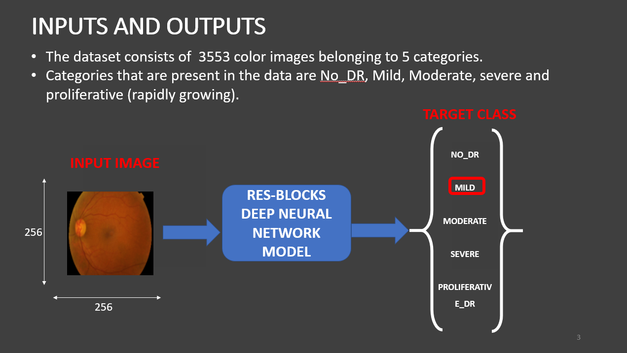
The dataset consists of 3553 colour images belonging to 5 categories.
Categories that are present in the data are: NO_DR, Mild, Moderate, severe, and proliferative

input

Importing Libraries

import pandas as pd
import numpy as np
import tensorflow as tf
from tensorflow import keras
import os
import matplotlib.pyplot as plt
import PIL
import seaborn as sns
from sklearn.model_selection import train_test_split
from sklearn.utils import shuffle
from tensorflow.keras.preprocessing.image import ImageDataGenerator
from tensorflow.keras.applications.resnet50 import ResNet50
from tensorflow.keras.applications.inception_resnet_v2 import InceptionResNetV2
from tensorflow.keras.layers import *
from tensorflow.keras.models import Model, load_model
from tensorflow.keras.initializers import glorot_uniform
from tensorflow.keras.utils import plot_model
from IPython.display import display
from tensorflow.keras import backend as K
from tensorflow.keras.optimizers import SGD
from tensorflow.keras.preprocessing.image import ImageDataGenerator
from tensorflow.keras.models import Model, Sequential
from tensorflow.keras.callbacks import ReduceLROnPlateau, EarlyStopping, ModelCheckpoint, LearningRateScheduler

Now I will set the style of the notebook to be monokai theme and this line of code is important to ensure that we are able to see the x and y axes clearly.If you don’t run this code line, you will notice that the xlabel and ylabel on any plot is black on black and it will be hard to see them.

from jupyterthemes import jtplot
jtplot.style(theme='monokai', context='notebook', ticks=True, grid=False) 

Listing down the images present in the training data

os.listdir('./train')
os.listdir(os.path.join('train', 'Mild'))

Checking the images in the dataset and returns the list of files in the folder, in this case image class names

train = []
label = []
for i in os.listdir('./train'):
  train_class = os.listdir(os.path.join('train', i))
  for j in train_class:
    img = os.path.join('train', i, j)
    train.append(img)
    label.append(i)

print('Number of train images : {} \n'.format(len(train)))

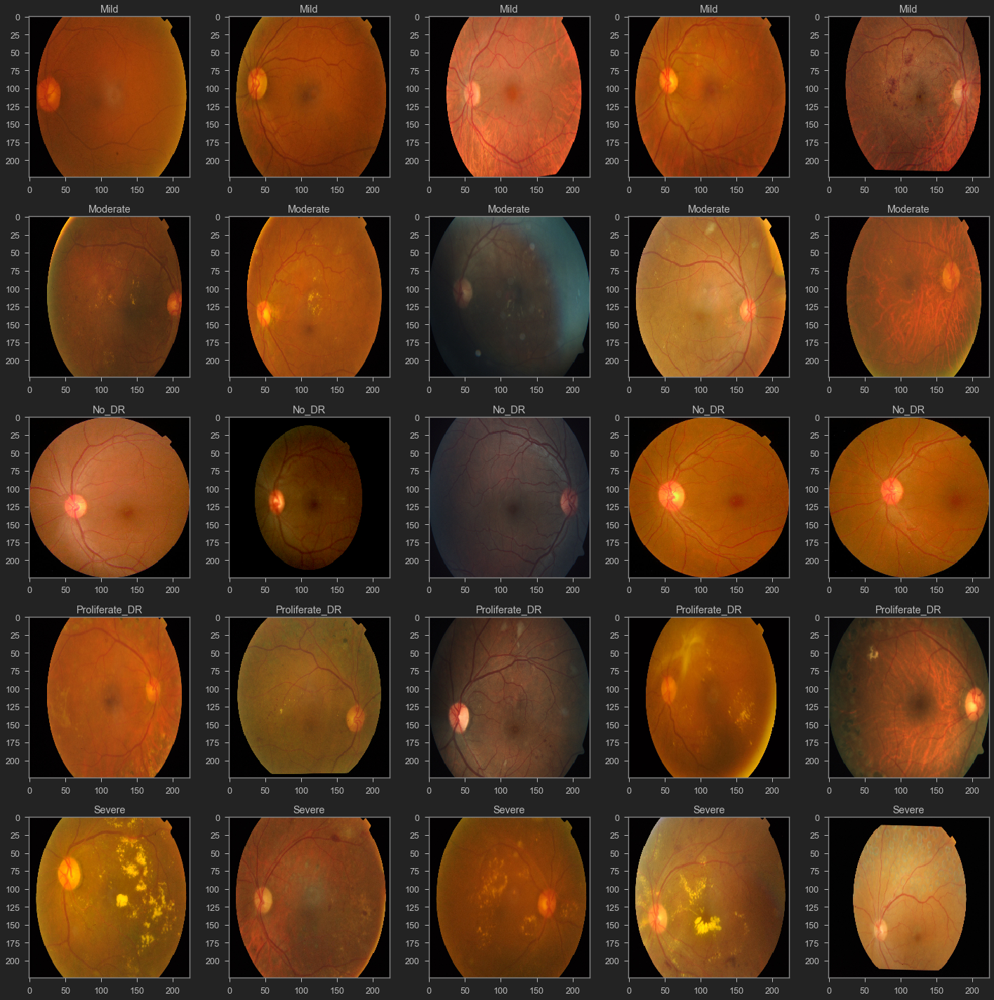
Performing Data Exploration and Data Visualisation

Visualize 5 images for each class in the dataset

fig, axs = plt.subplots(5, 5, figsize = (20, 20))
count = 0
for i in os.listdir('./train'):
  # get the list of images in a given class
  train_class = os.listdir(os.path.join('train', i))
  # plot 5 images per class
  for j in range(5):
    img = os.path.join('train', i, train_class[j])
    img = PIL.Image.open(img)
    axs[count][j].title.set_text(i)
    axs[count][j].imshow(img)  
  count += 1

fig.tight_layout()

input

Now we will check the number of images in each class in the training dataset

No_images_per_class = []
Class_name = []
for i in os.listdir('./train'):
  train_class = os.listdir(os.path.join('train', i))
  No_images_per_class.append(len(train_class))
  Class_name.append(i)
  print('Number of images in {} = {} \n'.format(i, len(train_class)))
retina_df = pd.DataFrame({'Image': train,'Labels': label})
retina_df

Perform Data Augumentation and create data generator

We will shuffle the data and split it into training and testing
Create run-time augmentation on training and test dataset
For training datagenerator, we add normalization, shear angle, zooming range and horizontal flip

retina_df = shuffle(retina_df)
train, test = train_test_split(retina_df, test_size = 0.2)
train_datagen = ImageDataGenerator(
        rescale = 1./255,
        shear_range = 0.2,
        validation_split = 0.15)

For test datagenerator, we only normalize the data.

test_datagen = ImageDataGenerator(rescale = 1./255)

Creating datagenerator for training, validation and test dataset.

train_generator = train_datagen.flow_from_dataframe(
    train,
    directory='./',
    x_col="Image",
    y_col="Labels",
    target_size=(256, 256),
    color_mode="rgb",
    class_mode="categorical",
    batch_size=32,
    subset='training')

validation_generator = train_datagen.flow_from_dataframe(
    train,
    directory='./',
    x_col="Image",
    y_col="Labels",
    target_size=(256, 256),
    color_mode="rgb",
    class_mode="categorical",
    batch_size=32,
    subset='validation')

test_generator = test_datagen.flow_from_dataframe(
    test,
    directory='./',
    x_col="Image",
    y_col="Labels",
    target_size=(256, 256),
    color_mode="rgb",
    class_mode="categorical",
    batch_size=32)

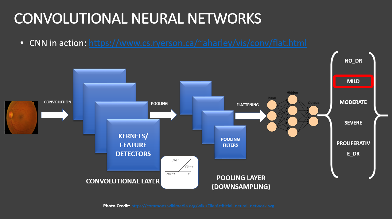
Understand the intuition behind Convolutional Neural Network (CNN)

A convolutional neural network, or CNN, is a deep learning neural network sketched for processing structured arrays of data such as portrayals.
CNN are very satisfactory at picking up on design in the input image, such as lines, gradients, circles, or even eyes and faces.
A convolutional neural network is a feed forward neural network, seldom with up to 20.
The strength of a convolutional neural network comes from a particular kind of layer called the convolutional layer.
CNN contains many convolutional layers assembled on top of each other, each one competent of recognizing more sophisticated shapes.
The agenda for this sphere is to activate machines to view the world as humans do, perceive it in a alike fashion and even use the knowledge for a multitude of duty such as image and video recognition, image inspection and classification, media recreation, recommendation systems, natural language processing, etc.

input

Why is ResNet (Residual Network) needed ?

As CNN began to grow deeper, the cause the vanishing gradient problem.
It occurs when the gradient is being backpropogated to earlier layers, it leads to smaller gradient.
Residual Network includes “skip connection” which enables traing of 152 layers without vanishing gradient problem.
They add identity mappings on top of CNN.

input

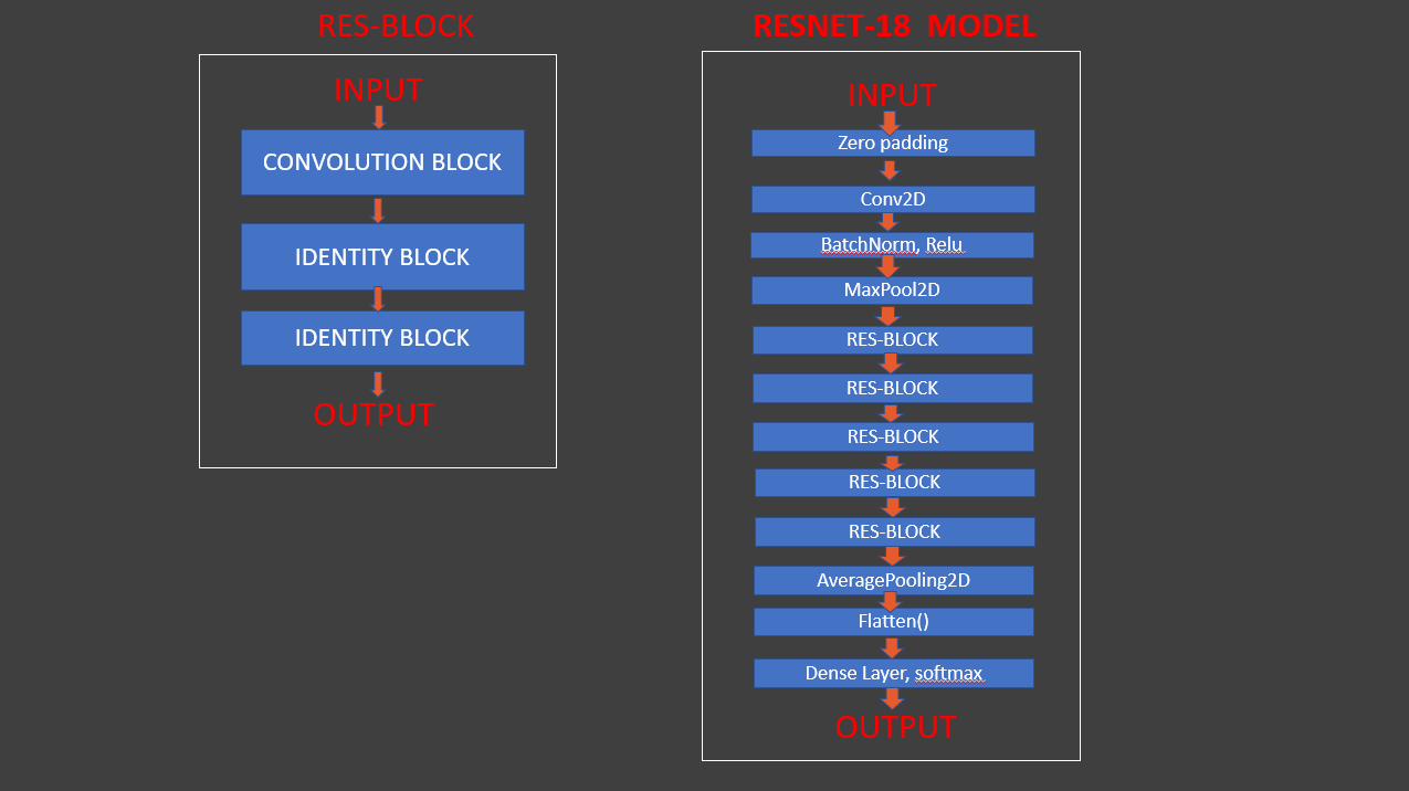
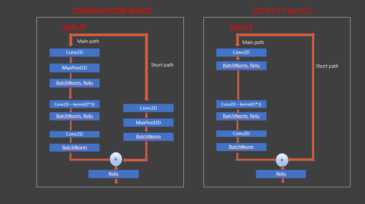
Build ResNet block based deep learning model

def res_block(X, filter, stage):
  
  # Convolutional_block
  X_copy = X

  f1 , f2, f3 = filter
    
  # Main Path
  X = Conv2D(f1, (1,1),strides = (1,1), name ='res_'+str(stage)+'_conv_a', kernel_initializer= glorot_uniform(seed = 0))(X)
  X = MaxPool2D((2,2))(X)
  X = BatchNormalization(axis =3, name = 'bn_'+str(stage)+'_conv_a')(X)
  X = Activation('relu')(X) 

  X = Conv2D(f2, kernel_size = (3,3), strides =(1,1), padding = 'same', name ='res_'+str(stage)+'_conv_b', kernel_initializer= glorot_uniform(seed = 0))(X)
  X = BatchNormalization(axis =3, name = 'bn_'+str(stage)+'_conv_b')(X)
  X = Activation('relu')(X) 

  X = Conv2D(f3, kernel_size = (1,1), strides =(1,1),name ='res_'+str(stage)+'_conv_c', kernel_initializer= glorot_uniform(seed = 0))(X)
  X = BatchNormalization(axis =3, name = 'bn_'+str(stage)+'_conv_c')(X)


  # Short path
  X_copy = Conv2D(f3, kernel_size = (1,1), strides =(1,1),name ='res_'+str(stage)+'_conv_copy', kernel_initializer= glorot_uniform(seed = 0))(X_copy)
  X_copy = MaxPool2D((2,2))(X_copy)
  X_copy = BatchNormalization(axis =3, name = 'bn_'+str(stage)+'_conv_copy')(X_copy)

  # ADD
  X = Add()([X,X_copy])
  X = Activation('relu')(X)

  # Identity Block 1
  X_copy = X


  # Main Path
  X = Conv2D(f1, (1,1),strides = (1,1), name ='res_'+str(stage)+'_identity_1_a', kernel_initializer= glorot_uniform(seed = 0))(X)
  X = BatchNormalization(axis =3, name = 'bn_'+str(stage)+'_identity_1_a')(X)
  X = Activation('relu')(X) 

  X = Conv2D(f2, kernel_size = (3,3), strides =(1,1), padding = 'same', name ='res_'+str(stage)+'_identity_1_b', kernel_initializer= glorot_uniform(seed = 0))(X)
  X = BatchNormalization(axis =3, name = 'bn_'+str(stage)+'_identity_1_b')(X)
  X = Activation('relu')(X) 

  X = Conv2D(f3, kernel_size = (1,1), strides =(1,1),name ='res_'+str(stage)+'_identity_1_c', kernel_initializer= glorot_uniform(seed = 0))(X)
  X = BatchNormalization(axis =3, name = 'bn_'+str(stage)+'_identity_1_c')(X)

  # ADD
  X = Add()([X,X_copy])
  X = Activation('relu')(X)

  # Identity Block 2
  X_copy = X


  # Main Path
  X = Conv2D(f1, (1,1),strides = (1,1), name ='res_'+str(stage)+'_identity_2_a', kernel_initializer= glorot_uniform(seed = 0))(X)
  X = BatchNormalization(axis =3, name = 'bn_'+str(stage)+'_identity_2_a')(X)
  X = Activation('relu')(X) 

  X = Conv2D(f2, kernel_size = (3,3), strides =(1,1), padding = 'same', name ='res_'+str(stage)+'_identity_2_b', kernel_initializer= glorot_uniform(seed = 0))(X)
  X = BatchNormalization(axis =3, name = 'bn_'+str(stage)+'_identity_2_b')(X)
  X = Activation('relu')(X) 

  X = Conv2D(f3, kernel_size = (1,1), strides =(1,1),name ='res_'+str(stage)+'_identity_2_c', kernel_initializer= glorot_uniform(seed = 0))(X)
  X = BatchNormalization(axis =3, name = 'bn_'+str(stage)+'_identity_2_c')(X)

  # ADD
  X = Add()([X,X_copy])
  X = Activation('relu')(X)

  return X

input_shape = (256,256,3)
X_input = Input(input_shape)
X = ZeroPadding2D((3,3))(X_input)

1 - stage

X = Conv2D(64, (7,7), strides= (2,2), name = 'conv1', kernel_initializer= glorot_uniform(seed = 0))(X)
X = BatchNormalization(axis =3, name = 'bn_conv1')(X)
X = Activation('relu')(X)
X = MaxPooling2D((3,3), strides= (2,2))(X)

2- stage

X = res_block(X, filter= [64,64,256], stage= 2)

3- stage

X = res_block(X, filter= [128,128,512], stage= 3)

4- stage

X = res_block(X, filter= [256,256,1024], stage= 4)

5- stage

X = res_block(X, filter= [512,512,2048], stage= 5) Average Pooling

X = AveragePooling2D((2,2), name = 'Averagea_Pooling')(X)
X = Flatten()(X)
X = Dense(5, activation = 'softmax', name = 'Dense_final', kernel_initializer= glorot_uniform(seed=0))(X)
model = Model( inputs= X_input, outputs = X, name = 'Resnet18')
model.summary()

Compile and train the deep learning model

model.compile(optimizer = 'adam', loss = 'categorical_crossentropy', metrics= ['accuracy'])
earlystopping = EarlyStopping(monitor='val_loss', mode='min', verbose=1, patience=15)
checkpointer = ModelCheckpoint(filepath="weights.hdf5", verbose=1, save_best_only=True)
history = model.fit(train_generator, steps_per_epoch = train_generator.n // 32, epochs = 1, validation_data= validation_generator, validation_steps= validation_generator.n // 32, callbacks=[checkpointer , earlystopping])
plt.plot(history.history['loss'])
plt.plot(history.history['val_loss'])
plt.title('Model loss')
plt.ylabel('loss')
plt.xlabel('epoch')
plt.legend(['train_loss','val_loss'], loc = 'upper right')
plt.show()

Evaluating the performance of the model

evaluate = model.evaluate(test_generator, steps = test_generator.n // 32, verbose =1)
print('Accuracy Test : {}'.format(evaluate[1]))

Assigning label names to the corresponding indexes

labels = {0: 'Mild', 1: 'Moderate', 2: 'No_DR', 3:'Proliferate_DR', 4: 'Severe'}

Now we load images and their predictions

from sklearn.metrics import confusion_matrix, classification_report, accuracy_score
# import cv2

prediction = []
original = []
image = []
count = 0

for item in range(len(test)):
  
  img= PIL.Image.open(test['Image'].tolist()[item])
  img = img.resize((256,256))
  image.append(img)
  img = np.asarray(img, dtype= np.float32)
  img = img / 255
  img = img.reshape(-1,256,256,3)
  predict = model.predict(img)
  predict = np.argmax(predict)
  prediction.append(labels[predict]) 
  original.append(test['Labels'].tolist()[item])

Now get the accuracy score

score = accuracy_score(original, prediction)
print("Test Accuracy : {}".format(score))

Finally Visualizing Results!

This brings us to the end of our project

import random
fig=plt.figure(figsize = (100,100))
for i in range(20):
    j = random.randint(0,len(image))
    fig.add_subplot(20, 1, i+1)
    plt.xlabel("Prediction: " + prediction[j] +"   Original: " + original[j])
    plt.imshow(image[j])
fig.tight_layout()
plt.show()

input